Resampling methods
This is the fourth in a series of posts that I’m doing on statistical learning. All the material is based on An Introduction to Statistical Learning book which was taught by the authors and Stanford University professors Trevor Hastie and Rob Tibshirani. The aim is to condense the concepts taught in the course and the material in the book to a series of under-10-minute reads.
This post is not supposed to be an exhaustive list of resampling methods, but only those mentioned in the book. These methods also happen to be the most commonly used ones.
Intro
When we build and train a statistical learning model, we can easily compute the prediction error rate on the data we used to train the model. This is not a good idea because our model has already seen the data and, therefore, it will in any case perform very well on predicting the response of this training data. If we choose a model based on this training error, we will most likely underestimate the true prediction error.
We can never really know the true prediction error. The test error error serves as a good proxy for the true prediction error. This is the error rate we get when we use our trained model to make predictions on data it has not seen, called “test data” or “holdout data”. Choosing a good model based on error and accuracy measures obtained from the test data usually serve as a reliable approximations of the performance of our model in the real world.
One way to find the test error rate is through statistical measures that try to estimate the test error from the training error. Common ones are Mallow’s $C_p$, Akaike information criterion ($AIC$), Bayesian information criterion ($BIC$), and Adjusted $R^2$. These are common and used by many statisticians and non-statisticians.
However, with advances in computational power, there are a number of newer, more reliable ways to estimate the test error.
Validation set approach
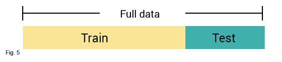
This is a simple approach where the full dataset is split into training and test sets. The model is first trained on the training set and tested on the test set. The performance of the model is evaluated on the basis of error and accuracy measures obtained from the test set.
However, in most cases, we do not have enough data to split into smaller subsets. Statistical learning algorithms perform best when trained on large datasets. Splitting the data in this way also means our final model will have larger than expected variance. A better approach is K-fold cross validation.
$K$-Fold cross validation
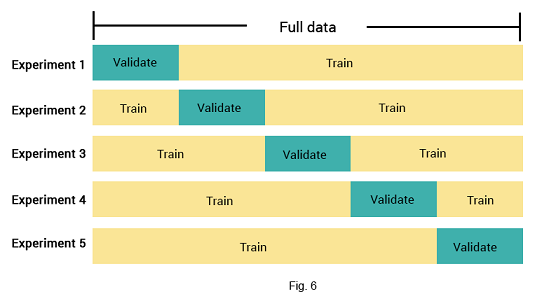
In K-fold cross validation (CV), the full dataset is split into $K$ parts. The model is trained on $K-1$ part and tested on the $k$th subset. This is done $K$ times. This is a common approach and, if done right, has been empirically proven to be a good method to approximate the true prediction error. The approach also makes use of the full dataset.
K-fold CV can be used to select the best model among a number of different models that range in flexibility. CV also allows us to estimate the other measures as well, e.g. the tuning parameter $\lambda$ in shrinkage methods.
Bootstrap
Although developed in late 60s, the bootstrap method of resampling has only recently begun to be commonly used by statisticians, particularly when attempting to estimate a given statistical measure such as median or standard error.
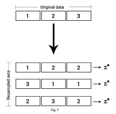
Bootstrap resampling takes our original dataset of size $n$ and creates $k$ random samples, each of size $n$, with replacement.1 Usually, $k = n$, i.e. we create $n$ random samples of size $n$. A given statistical measure $z$ is computed separately for each new sample and the results are averaged to get an estimate of the true population measure.2 In a similar fashion, the bootstrap method can also be used to estimate the accuracy of coefficient estimates of a linear regression model.
However, because it uses the same data, the bootstrap method greatly underestimates the true prediction error. This happens because our model will always yield higher test error when applied on unseen data. Bootstrap method also fails for a time-series data because of correlation. For example, the price of a stock on a given day is correlated to its price the previous day and there can only be one daily price. Because sampling is done randomly and with replacement, test statistics for the these samples obtained by bootstrap will be highly inaccurate in a time-series.
Nonetheless, it is still a good technique for estimating, e.g., standard errors of coefficient terms in a linear model or approximating confidence intervals of a population parameter.
FOOTNOTES
-
To understand what “replacement” means, think of a jar of three balls. Each time you pick a ball from the jar, you put back in. In resampling, this translates to: Each observation from the original dataset can appear twice or more in the sampled data. ↩
-
In statistics jargon, this measure is known as a test statistic which could be anything we interested in estimating, e.g. mean or median. In resampling we are trying to obtain an estimate of the population test statistic through the “sample” test statistic. ↩